StrokeLens EXPLAINABLE ML

AN EXPLAINABLE MACHINE LEARNING CASE STUDY

Predict.
Explain.
Understand.

Models that make predictions.
Explanations that make them useful.

Explore real classification benchmarks, SHAP feature contributions and a complete ML workflow. Stroke prediction is the case study. Explainable ML is the transferable skill.

Richard Huang / UCL · COMP0172 / Research portfolio

5,110Original dataset records
4Classification model families
1,022Held-out test records
10Input features

01 / MODEL PERFORMANCE COMPARISON

One score is never the full picture.

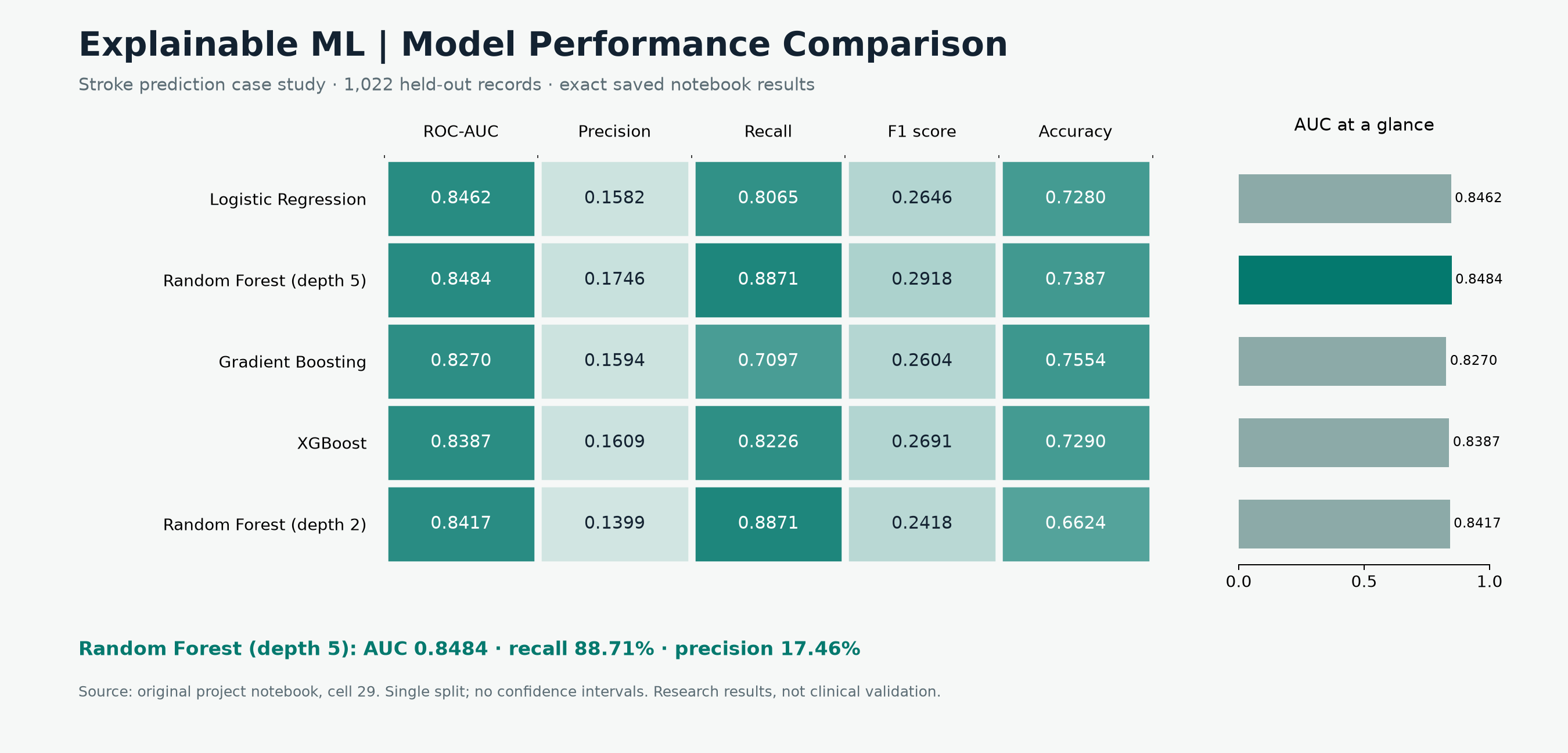
Five configurations. Five metrics. Actual saved results from the same held-out test set.

Download comparison chart ↓

Every model, every metric.

NOTEBOOK · CELL 29

Choose a metric column to explore it in the bar chart.

Model

Swipe the table horizontally to see all five metrics →

0.01.0Darker = higher value

Values shown to four decimal places. Color scale: 0–1 across all metrics. Metrics measure different properties and should not be averaged.

Download exact metrics CSV ↓
Compare one metric

0.000.250.500.751.00

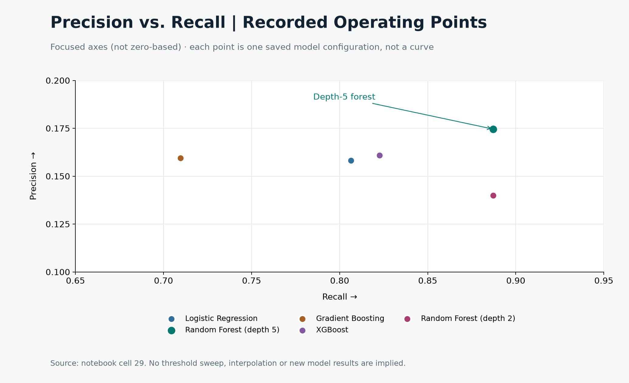
Precision vs. recall

↗ HIGHER ON BOTH AXES IS BETTER

Select a point or model name to inspect the recorded operating point.

Five saved operating points, not precision–recall curves. Switch between focused and full 0–1 axes. No threshold sweep is available.

Download precision–recall chart ↓
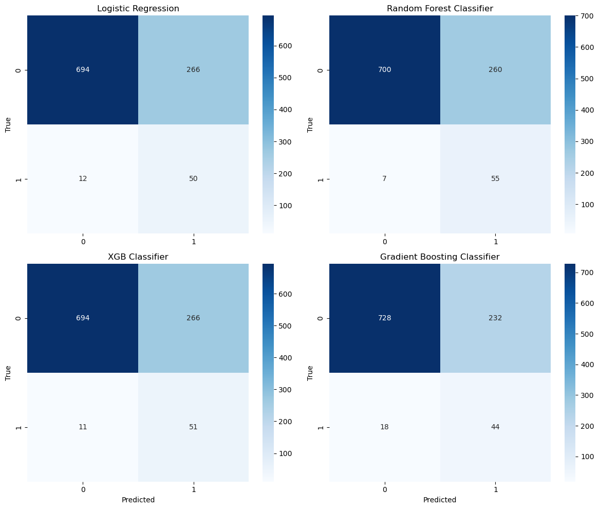
Inspect original confusion matrices and experiment context

Original notebook output, cell 31. Rows represent actual classes and columns predicted classes; class 1 denotes stroke. These figures cover the four primary classifiers.

Original four confusion matrices. Random Forest: 700 true negatives, 260 false positives, 7 false negatives and 55 true positives.

The notebook contains execution-state inconsistencies. This page faithfully presents its saved experiment outputs, rather than claiming a clean reproducible rerun.

Download original matrices ↓

02 / SHAP EXPLAINABILITY ANALYSIS

What moves a model’s prediction?

Explore feature importance, attribution direction and feature interactions in the original SHAP outputs.

EXPLAINABLE ML

THE IDEA BEHIND SHAP

Break an output into feature contributions.

Expected outputbaselineΣ SHAP valuesfeature contributionsModel outputin the explainer’s output space

Conceptual identity, not a patient-level explanation. For this notebook’s regressor, contributions are in model-output units, not log-odds or calibrated clinical risk.

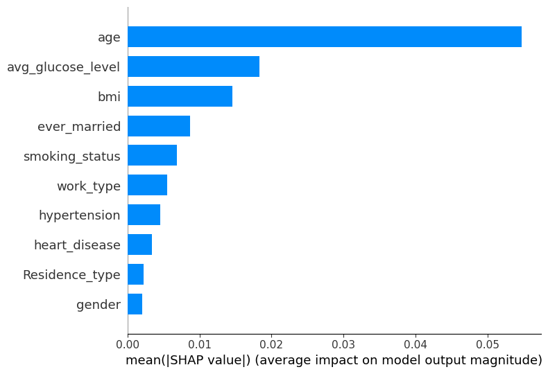
Original SHAP feature importance: age ranks first, followed by average glucose level and BMI.

Mean absolute SHAP values rank features by average contribution magnitude.

Explain the right model.

These plots explain the separate RandomForestRegressor in cell 34, using training data. They do not explain the benchmark classifier. This distinction is carried through the pipeline below.

Contribution is not causation.

SHAP describes learned associations. Correlated features and encoding choices affect attribution; a large SHAP value does not establish a causal effect or an actionable intervention.

Know the scope.

The repository provides saved global SHAP plots. Individual explanations would require per-row attribution values and the fitted model, which are not included in this repository.

03 / END-TO-END ML PIPELINE

From raw data to a reasoned result.

Follow the technical workflow. Select a stage to inspect its inputs, methods and outputs.

Download pipeline diagram ↓
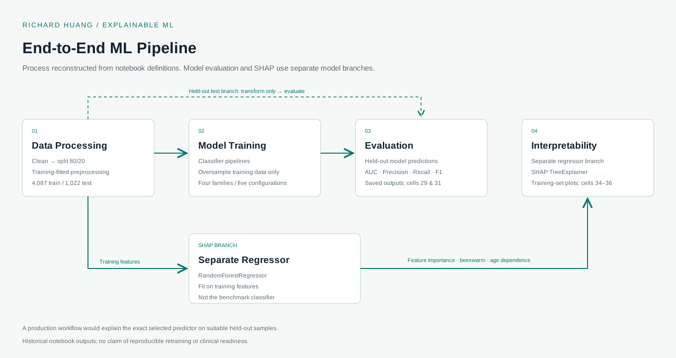
↳ TRAINING BRANCH Fit preprocessing & resampling on training data↳ HELD-OUT BRANCH Transform only → evaluate on 1,022 test records

STAGE 01 / DATA PROCESSING

Prepare the data. Protect the test set.

Remove ID and the single “Other” gender row, leaving 5,109 records. Split 80/20 with random_state=42. Fit mean BMI imputation on the training set and apply it to the test set.

Input
5,110 source records · 10 predictive features · stroke label
Methods
Pandas · train_test_split · SimpleImputer · OneHotEncoder · StandardScaler
Output
4,087 training rows / 1,022 test rows, with training-fitted transformations
Evidence
Notebook cells 3, 11 and 27. No stratify argument is set in the saved split code.
Two model branches, explicitly separated.

The classifier branch produces the performance benchmark. A separate regressor branch produces the saved SHAP plots. A production workflow would explain the exact selected predictor on suitable held-out samples.

Classifier pipelinesHeld-out performanceSeparate regressorTraining-set SHAP

04 / BEYOND THIS DATASET

Same ML questions. Different business decisions.

The methodology transfers. Every new use case needs its own data, model and validation.

APPLICATION EXAMPLES

HOW THE APPROACH COULD TRANSFER

Who might leave — and what drives the score?

Compare churn classifiers, inspect feature contributions and communicate the tradeoff between missing likely churners and contacting customers unnecessarily.

Predict

Classify likely churn

Explain

Attribute feature contributions

Evaluate

Test precision, recall & calibration

Would require: a churn-labeled dataset, a time-aware validation plan and experiments to establish whether a retention action works.

Illustrative application of the methodology. No client outcomes, commercial deployments or performance results are claimed for these examples.

Evidence first. Scope clearly stated.

This demo presents saved research results and original explanations. The notebook contains execution-state inconsistencies and no exported fitted model; this is not a reproducible retraining claim or a live prediction service. Clinical use would require reproducible training, calibration, subgroup testing and external validation. Not a medical device or diagnostic tool.

EXPLAINABLE ML / CLASSIFICATION / MODEL EVALUATION

Make your next model
easier to understand.

Explore my work in data science, interpretable machine learning and healthcare AI.

Visit Richard’s portfolio ↗